ClusteringAlgorithms
- MLModule
genre
authors
package
dll
definition
keywords
Purpose
The module ClusteringAlgorithms performs knowledge-independent clustering of arbitrary objects. You only need an affinity matrix encoding the similarity between the objects you desire to cluster.
In the special case of fiber clustering, the affinity matrix can be computed by the FeatureSpaceMatrix module or by the WeightMatrixByGrid module.
The module is based on the C Clustering Library for cDNA feature data (copyright (C) 2002 Michiel Jan Laurens de Hoon).
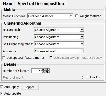
Usage
All the algorithms may use a feature space (FS) as an input. Most of them also support the input of a weight matrix.
If using a FS, only the first input is used.
If you would like to assign weights to the different features of the feature space you also need to check the box weightFeatures. Use the second input for the weight vector.
All algorithms which only require an affinity matrix also work if only the third input is used.
The first three algorithms (hierarchical), the last one of the partitioning-algorithms and all the algorithms capable of an automatic determination of the number of clusters (if useSpectralClustering is unchecked) are capable of calculating a weight matrix from FS. If you would like to use a weight matrix as an input you HAVE to check useWeights.
If you would like to cluster spectrally using a feature space you need to connect the first as well as the third input.
Details
Hierarchical
This class of algorithms creates a treelike structure in the first step. In a second step the tree is cut (starting at the root) until the desired number of clusters is obtained. The algorithms of this subgroup only differ by the method by which the degree of similarity between two knots is determined:
Complete: The most different elements belonging to two different knots are compared.
Average: The averages over all respective elements belonging to two different knots are compared.
Single: The most similar elements belonging to two different knots are compared.
Partitioning
The algorithms arbitrarily assign objects to clusters and compute a center of each cluster. Then they assign each object to the center which is most similar to it. The centers of every cluster are calculated again and the distances between the centers and the objects are computed; followed by another assignment of objects to centers. The whole procedure is repeated until all the centers are optimal and each object is assigned to the correspondingly nearest center.
Methods to compute the centers:
Means: average of the cluster elements (the center is not necessarily a real element of the cluster).
Median: median of the cluster elements (the center is not necessarily a real element of the cluster).
Medoid: The center always is a real element of the cluster: namely the element which yields the smallest total distance or the greatest total weight when summed over all other members of the cluster.
Since the clustering solution is very sensitive to the initial configuration of centers (which is initialized by a random number generator) the algorithm should be run several times (iterations) in order to find the best solution. The field ifound indicates how often the optimal solution has been found. If this number is low it is probable that there is a better solution available. The clusteringError is an output of the partitioning algorithms (high value means bad clustering). It is the sum of the distances of each object to the center of its cluster summed over all clusters.
Self-organizing maps
This algorithm uses a neural network. It maps points from the multi-dimensional feature space to a plane with a grid on top. The neural network searches for a map where the similarity of the results yielded by the neurons corresponds to the distances in the feature space. You can choose from several different metrics; i.e. different ways to measure a distance in the feature space.
Automatic
This algorithm clusters spectrally. It starts with two eigenvectors and assigns two centers. Then a third center is placed in the origin and the algorithm checks if any object should be assigned to the new center now. If any objects have been assigned to the new center, new, optimal centers are calculated; very much like in regular k-means clustering. Subsequently the algorithm adds a third eigenvector, a center is placed in the origin again and the algorithm checks if any objects have to be assigned to this new center and so on. The procedure is repeated until the cluster (newly centered in the origin) remains empty.
The internal algorithm for the computation of the centers is either elongated k-means or elongated k-medoids. Complete-linkage clustering is used to initialize the first two clusters to start with.
The field useFom only works when using a feature space. This so-called Figure of Merit can be utilized to estimate the quality of clustering and to check if the found number of clusters is plausible. If clusters are well separated all the features within each cluster correlate; i.e. each object of the same cluster has approximately the same coordinates in the feature space (tight clusters).
To calculate the FOM you have to cluster #dim(FS) times.
FOM = 0 if each object is assigned to its own separate cluster.
FOM = max if there is only one cluster.
You could try to determine the number of clusters using FOM. For this purpose you need to run FOM (number of different amounts of clusters you suspect dim(FS)) times: The idea is to omit one feature at a time (same for each object) and to cluster after the other features. In the end you calculate the clustering error with respect to the omitted feature and sum the errors for all omitted features (which is the actual FOM). In theory the number of clusters maximizing the curvature of a FOM versus the number of clusters is the number of choice.
Note: Calculating six FOMs takes about an hour!
FOM should work in theory but it is unclear if it really yields a plausible number of clusters. It is very expensive (therefore not really usable) and therefore to be treated with care!
Checking the box ‘Use spectral FS’ allows you to change the settings on the file card ‘Spectral Decomposition’.
If activated, a spectral feature space matrix is calculated either from a feature space or from an affinity matrix.
You can use different weights and metrics in order to compute the affinity matrix to be used in the singular value decomposition (SVD).
The spectral feature space matrix computed from the SVD is used to calculate the actual affinity matrix for clustering. Weighting the spectral feature space matrix has no point.
Windows
Default Panel
status
status showing some information
Input Fields
inputFeatureSpaceMatrix
- name: inputFeatureSpaceMatrix, type: MLBase
Feature space matrix for clustering, alternatively inputWeightMatrix can be used!
inputFeatureWeightVector
- name: inputFeatureWeightVector, type: MLBase
Vector used for weighting single features.
inputWeightMatrix
- name: inputWeightMatrix, type: MLBase
weight matrix which can directly be used for clustering
Output Fields
outObject
- name: outObject, type: MLBase
Vector indicating the clustering result
outCurve
- name: outCurve, type: MLBase
Out curve for eigenvalue regression where eigenvalues are plotted against their indices in the list of descending order. The x-axis shows the eigenvalue index (number of clusters), the y-axis shows the corresponding eigenvalues.
Parameter Fields
Visible Fields
Auto update
- name: autoUpdate, type: Bool, default: TRUE
If checked, the module computes anew on any input change.
Auto apply
- name: autoApply, type: Bool, default: TRUE
If checked, any parameter changes causes the module to compute anew.