HistogramSphereInterpolationPolynomial

MLModule

author	Tim Kroeger
package	FMEwork/Release
dll	MLStochasticCollocation
definition	MLStochasticCollocation.def
see also	TensorInterpolationPolynomial, SmolyakInterpolationPolynomial, EvaluateInterpolationPolynomial, DeriveInterpolationPolynomial, ScalePointInterpolationPolynomial, IntegrationInterpolationPolynomial, SimplifyInterpolationPolynomial, MultiplyInterpolationPolynomial, IntegrateBoxInterpolationPolynomial, CovarianceMatrixInterpolationPolynomial, PartiallyEvaluateInterpolationPolynomial, HistogramInterpolationPolynomial, Histogram3DInterpolationPolynomial, AddInterpolationPolynomial, SlightlySimplifyInterpolationPolynomial, TranslateInterpolationPolynomial, ImageListInterpolationPolynomial, GraphInterpolationPolynomial, InterpolatePolynomialToLinearFunction, FactorZeroInterpolationPolynomial
keywords	interpolation, polynomial, multivariate, histogram

Purpose

The module HistogramSphereInterpolationPolynomial computes (an approximation to) a histogram of a multivariate interpolation polynomial.

The histogram has values that are supposed to lie on the sphere S². Since S² is contained in the three-dimensional space, this polynomial is represented as three scalar-valued multivariate polynomials. The values do not have to exactly lie on the sphere (which is very unlikely anyway). Instead, they are internally projected onto the sphere.

In more detail, the module works as follows: The sphere is partitioned into two half-spheres, each of which is partitioned into a number of latitudes (given by the Number of Latitudes field, and each latitude is partitioned into a number of sectors (determined automatically such that they have approximately squared shape). The polynomial is evaluated at a number of points (depending on the Histogram Accuracy field), and each value is projected onto the sphere. For each sphere sector, the number of points whose values lie inside this sector is counted. This number is then divided by the number of evaluation points and the respective sector size. The result is the histogram. To display this histogram as an ML image, the center of each voxel is projected onto the sphere, and the voxel then gets the gray value of the sector its projected center lies in.

Windows

Default Panel

Input Fields

inputPolynomial1

name: inputPolynomial1, type: MLBase

inputPolynomial2

name: inputPolynomial2, type: MLBase

inputPolynomial3

name: inputPolynomial3, type: MLBase

Output Fields

output0

name: output0, type: Image

Parameter Fields

Field Index

Bounding Box Polynomial 1: String	Simplify polynomials: Bool
Bounding Box Polynomial 2: String	Sphere Radius: Double
Bounding Box Polynomial 3: String
Bounding Box Selection: Enum
Histogram Accuracy: Integer
Manual Bounding Box: String
Number of Latitudes: Integer
Number of Voxels: Integer

Visible Fields

Bounding Box Polynomial 1

name: autoBBox1, type: String, persistent: no

Shows the generic bounding box of the first polynomial.

This value can also be obtained with an EvaluateInterpolationPolynomial module.

Bounding Box Polynomial 2

name: autoBBox2, type: String, persistent: no

Shows the generic bounding box of the second polynomial.

This value can also be obtained with an EvaluateInterpolationPolynomial module.

Bounding Box Polynomial 3

name: autoBBox3, type: String, persistent: no

Shows the generic bounding box of the third polynomial.

This value can also be obtained with an EvaluateInterpolationPolynomial module.

Bounding Box Selection

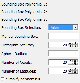
name: bBoxSelection, type: Enum, default: Union

Defines the bounding box mode.

Values:

Title	Name
Manual	Manual
Polynomial 1	Polynomial 1
Polynomial 2	Polynomial 2
Polynomial 3	Polynomial 3
Union	Union

Manual Bounding Box

name: manBBox, type: String

Sets a manual pre-image bounding box.

Histogram Accuracy

name: accuracy, type: Integer, default: 20, minimum: 2

Sets the number of points per space dimension in which the bounding box is scanned.

The higher the number, the better is the approximation of the histogram, but the slower is the computation.

Sphere Radius

name: sphereRadius, type: Double, default: 1

Sets the radius of the sphere along which you want to display your histogram.

Actually, this parameter only influences the world matrix of the image and the image scaling, nothing else. If you are confused, just leave the default, which is 1.

Number of Voxels

name: numVoxels, type: Integer, default: 20

Sets the number of voxels of the output ML image per space dimension.

The higher the number, the better the resolution. However, setting this to a high value and Histogram Accuracy to a low value will result it a very bad result (just try it and you will see).

Number of Latitudes

name: numLatitudes, type: Integer, default: 20

Sets the number of latitudes the sphere is partitioned into.

The higher the number, the better the resolution. However, setting this to a high value and Histogram Accuracy to a low value will result it a very bad result (just try it and you will see).

Simplify polynomials

name: simplifyPolynomials, type: Bool, default: FALSE

If checked, the polynomials will be simplified first.

This is the same procedure as in the SimplifyInterpolationPolynomial module.

This may either speed up or slow down the computation, depending on the polynomial and on the settings.

Note that simplifying a polynomial destroys the bounding box information, but that does not matter since this module evaluates the bounding boxes before simplifying.